Power Series Solutions IV - Analytic functions and ordinary points

#differential_equations

Our goal in this not is to give some type of answer to the question "When can we find a power series solution to a differential equation?" We begin by recalling a few basic facts about power series. We then analyze the case of second-order, linear, homogeneous differential equations. As we will eventually see, that situation is already complicated enough.

Analytic functions

There are two key properties of each power series: its center and its radius of convergence. A power series centered at $x = x_{0}$ is a series of the form

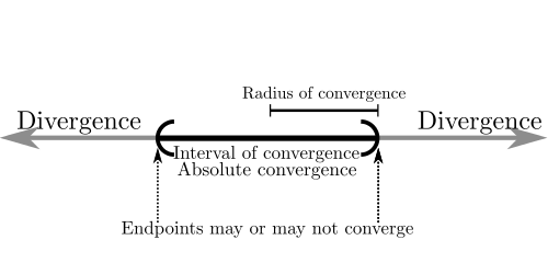
P (x) = \sum_{n = 0}^{\infty} a_{n} (x - x_{0})^{n} = a_{0} + a_{1} (x - x_{0}) + a_{2} (x - x_{0})^{2} + \dots

A big part of Calculus III is building up the machinery to make sense of power series as functions. One of the central results is that a power series defines a function whose domain is always an interval centered at $x_{0}$ , hence the name center. The radius $R$ of that interval of convergence is called the radius of convergence of the power series. If that radius is finite, then we are guaranteed that the series $P (x)$ converges absolutely for all values of $x$ in the open interval $(x_{0} - R, x_{0} + R)$ . The series might or might not converge at the endpoints. That depends on the particular series.

Part of the usefulness of power series is that "most" functions can be represented by power series, at least locally. More precisely, we say a function is analytic at $x_{0}$ if it can be represented by a power series near , i.e., if there is a power series $P (x)$ centered at such that $f (x) = P (x)$ for all in some open interval containing .

Warning

The word "analytic" can only be used to describe a function. It cannot be used to describe a differential equation.

In fact, we can say even more.

Taylor's Formula

If $f$ is analytic at $x_{0}$ , then $f$ is infinitely differentiable at $x_{0}$ and there is an open interval $I$ containing $x_{0}$ such that for all $x$ in $I$ one has

f (x) = \sum_{n = 0}^{\infty} \frac{f^{(n)} (x_{0})}{n!} (x - x_{0})^{n} .

In other words, if $f$ can be represented by a power series centered at $x_{0}$ , then there is only one possible such power series and its coefficients are given by the above formula. The most famous examples of these formulas are probably the following three Maclaurin series:

\begin{aligned} e^{x} & = \sum_{n = 0}^{\infty} \frac{1}{n!} x^{n} = 1 + x + \frac{1}{2!} x^{2} + \frac{1}{3!} x^{3} + \dots \\ \sin (x) & = \sum_{\begin{array}{c} n = 0 \\ n odd \end{array}}^{\infty} \frac{(- 1)^{(n - 1) / 2}}{n!} x^{n} = x - \frac{1}{3!} x^{3} + \frac{1}{5!} x^{5} + \dots \\ \cos (x) & = \sum_{\begin{array}{c} n = 0 \\ n even \end{array}}^{\infty} \frac{(- 1)^{n / 2}}{n!} x^{n} = 1 - \frac{1}{2!} x^{2} + \frac{1}{4!} x^{4} + \dots \end{aligned}

Each of these three equalities holds for all real $x$ , a fact that is not part of Taylor's formula above but is wonderful nonetheless. Another famous power series representation comes from the geometric series formula

\frac{1}{1 - x} = \sum_{n = 0}^{\infty} x^{n} = 1 + x + x^{2} + \dots

In contrast to the first three Maclaurin series, the above equality only holds for $x$ in the interval $(- 1, 1)$ . The function on the left is defined for all $x \neq 1$ , but it only agrees with the power series on the right on the interval $(- 1, 1)$ , which happens to be the interval of convergence of that power series. What could we say about the function on the left at a point like $x = 2$ ? Taylor's Formula gives us the recipe for the only possible power series centered at $x = 2$ that could represent it. It turns out that we have

\frac{1}{1 - x} = \sum_{n = 0}^{\infty} (- 1)^{n + 1} (x - 2)^{n} = - 1 + (x - 2) - (x - 2)^{2} + \dots,

with equality holding for all $x$ in the interval $(1, 3)$ .

At this point you might be wondering how to tell when a given function $f$ is analytic at a point $x = x_{0}$ . Technically, the answer is that the function $f$ must satisfy two properties: first, $f$ must be infinitely differentiable at $x_{0}$ ; second, the function $f$ must agree with its Taylor series centered at $x_{0}$ on some open interval around $a$ . This is not always easy to verify, although you may have learned how to do so in Calculus III using Taylor's Remainder Estimate.

Fortunately there's good news. As far as we're concerned, "most" functions that we deal with are analytic at all points in their domain. Polynomials are analytic everywhere. So are the functions $e^{x}$ , $\sin (x)$ and $\cos (x)$ . Products of analytic functions are analytic, as are sums and differences. And ratios of analytic functions are analytic everywhere they're defined, i.e., everywhere except where the denominator vanishes. For our purposes we are going to be mostly concerned with rational functions, which are ratios of polynomials. For those functions, we conveniently have the following result.

Radius of convergence for rational functions

Suppose $f (x) = \frac{g (x)}{h (x)}$ , where $g$ and $h$ are polynomials with no common zeroes. Let $x_{0}$ be any points where $h (x_{0}) \neq 0$ . Then $f$ is analytic at $x_{0}$ , and the power series representation for $f$ at $x_{0}$ has radius of convergence $R$ , where $R$ is the minimum distance (in the complex plane) from $x_{0}$ to the zeroes of $h$ .

The zeroes of the denominator $h$ are called the poles of $f$ . If we choose a center $x_{0}$ for our power series representation of $f$ , then the radius of convergence of that series is the distance from $x_{0}$ to the nearest pole of $f$ .

Example

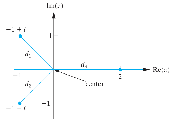
Consider the function

f (x) = \frac{x - 1}{(x^{2} + 2 x + 2) (x - 2)} .

Using the quadratic formula, the poles of $f$ are at $x = 2$ and $x = - 1 \pm i$ . It follows that $f$ is analytic at every point except those three. In particular, it is analytic at 0 and the radius of convergence for the corresponding Taylor series is the minimum distance from 0 to those three poles.

Using the distance formula, the distances from 0 to those three poles are 2, $\sqrt{2}$ , and $\sqrt{2}$ , respectively, so the minimum distance from 0 to any of the poles is $\sqrt{2}$ . By our above theorem, the Maclaurin series for $f$ thus has radius of convergence $R = \sqrt{2}$ .

Note

The best part of the above theorem is that it tells us radii of convergence without having to work out explicit formulas for Taylor series and then run Ratio Tests, computations that could be exceedingly tedious.

Ordinary points of differential equations

For reasons that will become clear, we will restrict our attention to second-order, linear, homogeneous differential equations. Every such differential equation can be written in the form

y^{″} + p (x) y^{'} + q (x) y = 0.

We call this the standard form of the differential equation.

Note

You don't have to put your differential equation into standard when solving for a power series solution. This form is only needed when analyzing the differential equation, to determine whether looking for a power series solution is a good idea.

We can now answer the following:

Question

For which points $x_{0}$ does this differential equation possess a solution that is analytic at $x_{0}$ , i.e., that can be represented by a power series centered at $x_{0}$ ?

The following theorem gives sufficient (but not necessary) conditions to guarantee success:

Radius of convergence of power series solutions

Suppose $p$ and $q$ are analytic at $x_{0}$ Then the general solution to the differential equation

y^{″} + p (x) y^{'} + q (x) y = 0

is analytic at $x_{0}$ . Moreover, the radius of convergence of the general power series solution is at least as large^[1] as the minimum of the radii of convergence for the power series representations of $p$ and $q$ .

In other words, as long as the coefficient functions $p$ and $q$ are analytic at our chosen center $x_{0}$ , then so is the general solution. And that means we can find it using our power series method. Let's introduce a new term to describe this situation.

Definitions of ordinary and singular points

Consider the differential equation

y^{″} + p (x) y^{'} + q (x) y = 0.

We say $x_{0}$ is an ordinary point of the differential equation if both $p$ and $q$ are analytic at $x_{0}$ . We say $x_{0}$ is a singular point of the differential equation if either $p$ or $q$ (or both!) is not analytic at $x_{0}$ .

Warning

Again note that a differential equation cannot be said to be analytic. The word "analytic" only applies to a function.

Example

Consider the differential equation we first looked at when trying for a power series solution:

y^{″} + y = 0.

This differential equation is already in standard form, so the coefficient functions are the constant functions $p (x) = 0$ and $q (x) = 1$ . Since constant functions are analytic everywhere, this means every point $x_{0}$ is an ordinary point of this differential equation. By our theorem above, it follows that the general solution is analytic everywhere, as well, so we could find it using a power series (centered at wherever we liked). Moreover, the radii of convergence for the power series representations of $p$ and $q$ are both infinity, so the general solution to our differential equation is guaranteed to also have infinite radius of convergence.

Note

Polynomials can be viewed as finite power series. Since polynomials are defined everywhere, they have infinite radius of convergence when viewed as power series.

Example

Our second example earlier was the differential equation below, which is also already in standard form:

y^{″} + (2 - 4 x^{2}) y^{'} - 8 x y = 0.

Here we see $p (x) = 2 - 4 x^{2}$ and $q (x) = - 8 x$ . Both coefficient functions are polynomials and hence are analytic everywhere, with infinite radii of convergence. So once again every point $x_{0}$ is an ordinary point of the differential equation, and the general solution can be represented by a power series (with infinite radius of convergence) centered at whichever point $x_{0}$ we desire.

Example

Consider the differential equation

(1 - x^{2}) y^{″} - 2 x y^{'} + 6 y = 0.

In standard form, this differential equation is

y^{″} - \frac{2 x}{1 - x^{2}} y^{'} + \frac{6}{1 - x^{2}} y = 0,

so $p (x) = - \frac{2 x}{1 - x^{2}}$ and $q (x) = \frac{6}{1 - x^{2}}$ . These coefficient functions are both analytic everywhere except $x = \pm 1$ . In our new terminology, we can say that every $x_{0}$ other than $\pm 1$ is an ordinary point of the differential equation, while $x_{0} = 1$ and $x_{0} = - 1$ are singular points. For a specific example, the point $x_{0} = 0$ is an ordinary point of the differential equation, and the power series representations for $p$ and $q$ centered at 0 have radii of convergence 1. By our above theorem, it follows that the general solution to this differential equation can be represented by a power series centered at 0 with radius of convergence at least 1.

There are a few items worth stressing here. First, we should be very clear what our theorem does and does not say. It does say that if $x_{0}$ is an ordinary of the differential equation, then it is guaranteed that the general solution to the differential equation can be represented by a power series centered at $x_{0}$ . It does not say that if $x_{0}$ is a singular point of the differential equation, then there does not exist a solution to the differential equation that can be represented by a power series centered at $x_{0}$ . It could still happen, it's just no longer guaranteed. We will see what can go wrong, and how things could still go right.

What can possibly go wrong?

Consider the differential equation

4 x^{2} y^{″} - (3 + 4 x) y = 0.

In standard form, this differential equation is

y^{″} - \frac{3 + 4 x}{4 x^{2}} y = 0,

so the coefficient functions are $p (x) = 0$ and $q (x) = - \frac{3 + 4 x}{4 x^{2}}$ . The first is analytic everywhere, while the second is analytic everywhere except at $x_{0} = 0$ . So $x_{0} = 0$ is a singular point of this differential equation. This means we are not guaranteed we will can find a power series solution centered at 0. Let's try to find one anyway.

We will look for all solutions of the form $y = \sum_{n = 0}^{\infty} a_{n} x^{n}$ . If we substitute this into the left side of the current (standard) form of our differential equation, we will find

y^{″} - \frac{3 + 4 x}{4 x^{2}} y = \sum_{n = 2}^{\infty} n (n - 1) a_{n} x^{n - 2} - \frac{3 + 4 x}{4 x^{2}} \sum_{n = 0}^{\infty} a_{n} x^{n} .

Let's pause for a moment and imagine how this is about to play out. We need to perform some basic arithmetic, reindex some series, and then combine like powers of $x$ to obtain a single power series. A power series is a linear combination of nonnegative integer powers of $x$ , which means everything in our expression must be expressed as combinations of nonnegative integer powers of $x$ . Expressions like $\frac{3 + 4 x}{4 x^{2}}$ are not allowed, so they must be dealt with somehow. We essentially have three options:

Option 1

Algebraically manipulate the differential equation before substituting in our power series. In our current case, we could go back to the original version of the differential equation.

Option 2

Algebraically manipulate the offending expressions so as to rewrite them as linear combinations of powers of $x$ . In our current example, we could write $\frac{3 + 4 x}{4 x^{2}} = \frac{3}{4} x^{- 2} + x^{- 1}$ . In this case we've introduced negative powers of $x$ , but it turns out that this is okay and everything will work out fine.

Option 3

Replace every offending expression with its corresponding power series. For example, if there had been an $e^{x}$ in our differential equation, we could replace it with its Maclaurin series. This is usually the most computationally painful option.

For this example let's go with the first option, and plug our generic power series into the original differential equation. We find

\begin{aligned} 4 x^{2} y^{″} - (3 + 4 x) y & = 4 x^{2} \sum_{n = 0}^{\infty} n (n - 1) a_{n} x^{n - 2} - (3 + 4 x) \sum_{n = 0}^{\infty} a_{n} x^{n} \\ = \sum_{n = 2}^{\infty} 4 n (n - 1) a_{n} x^{n} - \sum_{n = 0}^{\infty} 3 a_{n} x^{n} - \sum_{n = 0}^{\infty} 4 a_{n} x^{n + 1} \\ = \sum_{m = 2}^{\infty} 4 m (m - 1) a_{m} x^{m} - \sum_{m = 0}^{\infty} 3 a_{m} x^{m} - \sum_{m = 1}^{\infty} 4 a_{m - 1} x^{m} \\ = \underset{m = 0}{\underset{⏟}{- 3 a_{0}}} + \underset{m = 1}{\underset{⏟}{(- 3 a_{1} - 4 a_{0}) x}} + \sum_{m = 2}^{\infty} (4 m (m - 1) a_{m} - 3 a_{m} - 4 a_{m - 1}) x^{m} \end{aligned}

So, $y$ is a solution of our differential equation exactly when

\begin{aligned} m = 0 : & - 3 a_{0} = 0 \\ m = 1 : & - 3 a_{1} - 4 a_{0} = 0 \\ m \geq 2 : & 4 m (m - 1) a_{m} - 3 a_{m} - 4 a_{m - 1} = 0. \end{aligned}

The first two equations give $a_{0} = 0$ and $a_{1} = - \frac{4}{3} a_{0} = 0$ . The last equation can be solved for $a_{m}$ to give

a_{m} = \frac{4}{4 m (m - 1) - 3} a_{m - 1}

for every $m \geq 2$ . In particular, each $a_{m}$ is a multiple of the coefficient before it. Since $a_{0} = 0$ and $a_{1} = 0$ , it now follows that every $a_{m} = 0$ . Thus, the only power series solution centered at 0 is

y (x) = 0 + 0 \cdot x + 0 \cdot x^{2} + \dots,

i.e., the trivial solution $y (x) = 0$ .

Warning

We will see in the next chapter that it can be critically important when solving a recursion equation like the one above to check to see if we have any danger of dividing by zero. For this equation, that amounts to asking whether there are any values of $m$ for which $4 m (m - 1) - 3 = 0$ . One can quickly find that the roots of this equation are $m = \frac{3}{2}$ and $m = - \frac{1}{2}$ . Since we are only considering integers $m \geq 2$ , there is no danger here for us.

For a linear, homogeneous differential equation, this is the only thing that can "go wrong" when looking for a power series solution centered at 0. The trivial solution is always a solution, and in this case it was the only solution that could be represented by a power series centered at 0. Nothing especially catastrophic has happened, other than us wasting our time and coming up empty handed. If you're a pessimist, this is what you should expect to happen when your desired center is a singular point of the differential equation. In the next example, however, we will see that this is always a chance that things might still work out.

So you're saying there's a chance

Let's take a look at the differential equation

x^{2} y^{″} + x y^{'} - (1 + x) y = 0.

In standard form this differential equation is

y^{″} + \frac{1}{x} y^{'} - \frac{1 + x}{x^{2}} y = 0,

so we can see that $x_{0} = 0$ is a singular point of this differential equation. Remember, this only means we are not guaranteed we can find a power series solution centered at 0, but there might be one. So let's look and see. As usual, we'll substitute our general power series centered at 0 into the left side of the differential equation and then simplify:

\begin{aligned} x^{2} y^{″} + x y^{'} - (1 + x) y & = x^{2} \sum_{n = 2}^{\infty} n (n - 1) a_{n} x^{n - 2} + x \sum_{n = 1}^{\infty} n a_{n} x^{n - 1} - (1 + x) \sum_{n = 0}^{\infty} a_{n} x^{n} \\ = \sum_{n = 2}^{\infty} n (n - 1) a_{n} x^{n} + \sum_{n = 1}^{\infty} n a_{n} x^{n} - \sum_{n = 0}^{\infty} a_{n} x^{n} - \sum_{n = 0}^{\infty} a_{n} x^{n + 1} \\ = \sum_{m = 2}^{\infty} m (m - 1) a_{m} x^{m} + \sum_{m = 1}^{\infty} m a_{m} x^{m} - \sum_{m = 0}^{\infty} a_{m} x^{m} - \sum_{m = 1}^{\infty} a_{m - 1} x^{m} \\ = \underset{m = 0}{\underset{⏟}{- a_{0}}} + \underset{m = 1}{\underset{⏟}{(a_{1} - a_{1} - a_{0}) x}} + \sum_{m = 2}^{\infty} (m (m - 1) a_{m} + m a_{m} - a_{m} - a_{m - 1}) x^{m} \\ = - a_{0} - a_{0} x + \sum_{m = 2}^{\infty} ((m^{2} - 1) a_{m} - a_{m - 1}) x^{m} . \end{aligned}

So, our power series is a solution exactly when the following equations are satisfied:

\begin{aligned} m = 0 : & - a_{0} = 0 \\ m = 1 : & - a_{0} = 0 \\ m \geq 2 : & (m^{2} - 1) a_{m} - a_{m - 1} = 0. \end{aligned}

The first two equations both imply $a_{0} = 0$ . We then find

\begin{aligned} m = 2 : & a_{2} = \frac{1}{3} a_{1} \\ m = 3 : & a_{3} = \frac{1}{8} a_{2} = \frac{1}{8 \cdot 3} a_{1} \\ m = 4 : & a_{4} = \frac{1}{15} = \frac{1}{15 \cdot 8 \cdot 3} a_{1} \\ ⋮ \end{aligned}

Thus, all power series solutions centered at 0 are of the form

\begin{aligned} y (x) & = 0 + a_{1} x + \frac{1}{3} a_{1} x^{2} + \frac{1}{24} a_{1} x^{3} + \frac{1}{360} a_{1} x^{4} + \dots \\ = a_{1} \underset{y_{1} (x)}{\underset{⏟}{(x + \frac{1}{3} x^{2} + \frac{1}{24} x^{3} + \frac{1}{360} x^{4} + \dots)}} \end{aligned}

While we didn't find two linearly independent solutions to our differential equation, we did at least find one, which is certainly better than nothing! In the next note we will see how to find another solution, which is something a little more general than a power series.

Suggested next notes

Frobenius Series Solutions I - Slightly generalizing power series

We will see examples for which the power series solution has a larger radius of convergence than either $p$ or $q$ . ↩︎